Graphs and Trees are at the heart of a computer and very useful in representing and resolving many real world problems like calculating the best paths between cities (Garmin, TomTom) and other famous ones like Facebook search and Google search engine crawling. If you know any programming language, you might have heard of garbage collection and for that the typical graph search called Breadth First Search is used. In this post, I will try to cover the following topics.
- Graphs – directed, undirected and special case of directed which are called Directed Acyclic Graph(DAG)
- Trees – Binary trees and also most useful version of it, the Binary Search Trees (BST)
- Standard traversal techniques – Breadth First Search (BFS), Depth First Search (DFS).
I know it will be a bit lengthy but I assure you it will be worth going through. I will try to cover the following topics in another post.
- Overview of shortest path algorithms – BFS, Dijkstra and Bellman Ford
- BST Search, Pre-order, In-order and Post-order.
Graphs
A graph consists of vertices (nodes) and edges. Think vertex as a point or place and the edge is the line/path connecting two vertices. In a typical graph and tree nodes there will be some kind of information is stored and the vertices will be associated with some cost. There are mainly two types of graphs and they are undirected and directed graphs.
In undirected graphs, all of the edges are undirected which means we can travel in either direction. So if we have an edge between vertex A and B, then we can travel from A to B and also from B to A. Following is the sample undirected graph.
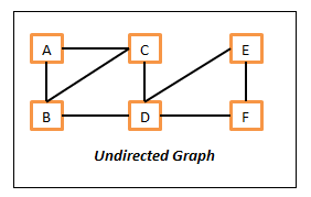
A Undirected Graph
Here in this undirected graph,
- The vertices are – A, B, C, D, E and F.
- The edges are – {A, B}, {A, C}, {B, C}, {B, D}, {C, D}, {D, E}, {D, F} and {E, F}. Here edge {A, B} means, we can move from A to B and also from B to A.
In directed graphs, all of the edges are directed which means we can only travel in the direction of an edge. So for example, if we have an edge between vertices A and B, then we can only go from A to B and not from B to A. If we need to go from B to A, then there should be another edge which should point B to A. Following is the sample directed graph.
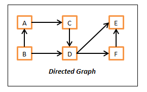
Directed Graph
Here in this directed graph,
- The vertices are – A, B, C, D, E and F.
- The edges are – (A, C), (B, A), (B, D), (C, D), (D, E), (D, F) and (F, E). Here edge (A, C) means, we can only move from A to C and not from C to A.
The graphs can be mixed with both directed and undirected edges but let us keep this aspect away in this post to understand the core concepts better. Just an FYI the undirected edges are represented by curly braces ‘{}’ where as directed edges are represented by ‘()’.
Directed Acyclic Graphs – DAG
This is a variation of standard directed graph without any cycle paths. It means there is no path where we can start from a vertex and comeback to the same starting vertex by following any path. By the way, cycles in the graph are very important and we need to be very careful about it. Otherwise, we could end up writing infinite algorithms which will never be completed.

The above diagram does not have a cycle, so it is a DAG. Basically we can start from any node and won’t come back to the same starting node.

If we carefully look at the above listed directed graph, there is a cycle path and because of that, this graph is not a DAG. We can start from node A and come back to it by following the path.
Trees
This is another variation or we may call it subset of a graph. So we can say, all trees are graphs but not all graphs are trees. It is almost similar to the real world tree. It will have one top level vertex which is called root, and every node will have either zero or more child vertices. The best examples of tree data structure are family relationship and a company organization chart. Few important things to note down here,
- There will not be any cycles in this.
- Every node will have only one parent except the root which will not have any.
Following is a sample tree structure.
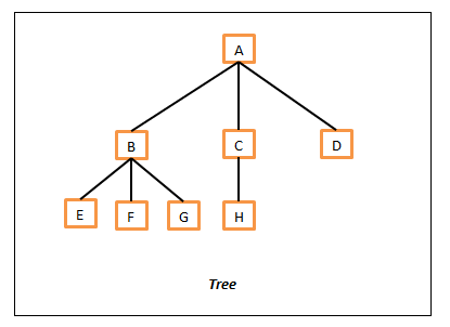
A Tree
As a standard the tree is represented from top to bottom. In this, the top node A is called as root of this tree as there are no parents to it. Then all of the child vertices (B, C and D) of A are represented on next level. All of the nodes which don’t have any child nodes (E, F, G, H and D) are called leaf nodes.
DAG vs Tree
As you can see by now both the DAG and tree will not have any cycle paths but there is a key difference that is, in DAG there can be nodes with multiple parents but where as in tree, every node will have either a single parent or none. Following diagrams depicts this difference.
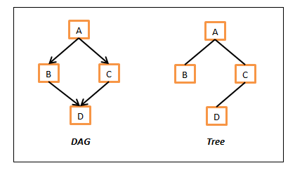
DAG vs Tree
In the above DAG example, D has two parents B and C and this is not possible in the tree. In tree example above, D has just one parent C.
Binary Tree
This is a version of the tree structure and in this every node can have strictly at most two child nodes. That means a node either can have two child nodes, just one or simply no child nodes in which case we call them leaf nodes. Following is a sample binary tree.
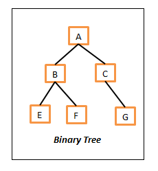
Binary Tree
Binary Search Tree (BST)
This is a most useful version of the Binary Tree in which every node (including root) holds the following two properties.
- The left child node (if exists) should contain the value which is less than or equal to the parent.
- The right child node (if exists) should contain the value which is greater than or equal to the parent.
The above ordering property is really useful which we can understand clearly when we go through some of the search algorithms (especially the Binary search).
For simplicity, we will use the numbers in the nodes to show this relationship but the nodes can contain any information as long they are comparable. That means we should be able to compare them in some way and tell, whether those are equal or whether which one is greater. Following is a sample BST,
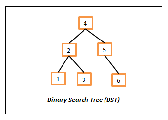
Binary Search Tree
Data Structure representation
Hopefully all of the above details provide the insights on graphs and tree data structures. Before we get on to the actual traversals and searching algorithms, it is essential and useful to understand how they are represented or stored them in programming languages.
Following are the two mostly used representations.
Adjacency Lists
In this, the node is represented by an object and the edge is represented by the object references. Every object will have some data and a list of adjacent node references or a method which can return the list of adjacent nodes. If there are no neighbors, then it will be null or empty. So in nutshell, we have some mechanism to quickly find out neighbors for a given node.
There is also another way to represent using adjacency lists which having a map which contains the key as the node and the value is list containing all of its neighbors. In this case, we can simply get all of its neighbors of a node N by simply looking for a key N in the map. That is we could say the neighbors of node N are simply Adj[N] where Adj is the adjacency map. Following is a sample representation of this representation.
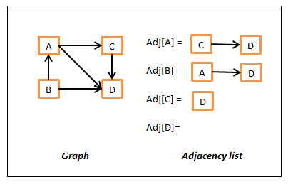
Graph Adjacency list representation
Matrix representation
In this, we will use a double dimensional array where rows and columns represent the nodes and will use some kind of special value or actual edge cost as the value if they are connected. Following is sample example of representation.
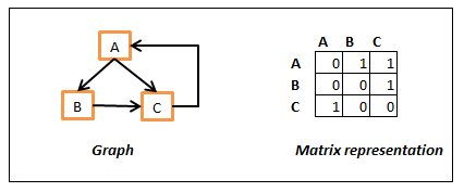
Graph matrix representation
In the above, we have used 1 to represent the edge and 0 for no edge and we are looking from row to column. That is Array[B][C] is 1 as there is edge from B to C but Array[C][B] is zero as there is no edge between C to B. We could also use some value to represent the actual cost and use some sentinel (infinity or -1) value to represent no connection between the nodes. Yes, it is not a regulatory object oriented design but it have its own advantages like accessing random node and get the edge cost of a neighbor in constant time.
Searching Algorithms
There are two main search techniques which work fine on both the graphs and all versions of trees. It is just that we need to be careful about the cycles in graphs.
Breadth First Search (BFS)
In this, we will search or examine all of the sibling nodes first before going to its child nodes. In other words, we start from the source node (root node in trees) and visit all of the nodes reachable (neighboring nodes) from the source. Then we take each neighbor node and perform the same operation recursively until we reach destination node or till we run out of graph. The following color coded diagrams depicts this searching.
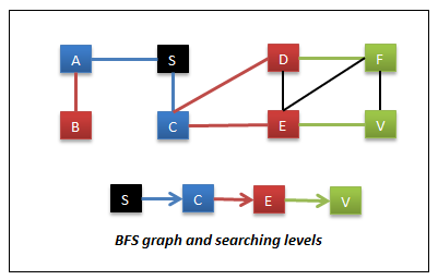
Breadth First Search
In this, the starting node is S and the target node is V. In this,
- Visit all of the nodes reachable from S. So we visit nodes A & C. These are the nodes reachable in 1 move or nodes at level 1.
- Then visit the nodes reachable from A & C. So we visit nodes B, D & E. These are the nodes reachable in 2 moves or we can say nodes at level 2.
- Then visit the nodes reachable from B, D & E. So we visit nodes F & V. These are the nodes reachable in 3 moves or we can say at level 3.
Advantages of this approach are,
- The path from which we first time reach a node can be considered as shortest path if there are no weights/costs to the edges or they might be constant. This is called single source shortest paths.
- This can be used in finding friends in social network sites like Facebook, Google+ and also linked in. In linked in, you might have seen the 1st, 2nd or 3rd degree as super scripts to the friend’s names – it means that they are reachable in 1 move, 2 moves and 3 moves from you and now you might guess how they calculate that J
BFS implementation
We can implement this in multiple ways. One of the most popular ways is by using Queue data structure and other by using lists to maintain the front and next tier nodes. Following is the java implementation of this algorithm.
public static void graphBFSByQueue(Node<String> source) {
//if empty graph, then return.
if (null == source) {
return;
}
Queue<Node<String>> queue = new LinkedList<Node<String>>();
//add source to queue.
queue.add(source);
visitNode(source);
source.visited = true;
while (!queue.isEmpty()) {
Node<String> currentNode = queue.poll();
//check if we reached out target node
if (currentNode.equals(targetNode)) {
return; // we have found our target node V.
}
//Add all of unvisited neighbors to the queue. We add only unvisited nodes to avoid cycles.
for (Node<String> neighbor : currentNode.neighbors) {
if (!neighbor.visited) {
visitNode(neighbor);
neighbor.visited = true; //mark it as visited
queue.add(neighbor);
}
}
}
}
public static void graphBFSByLevelList(Node<String> source) {
//if empty graph, then return.
if (null == source) {
return;
}
Set<Node<String>> frontier = new HashSet<Node<String>>();
//this will be useful to identify what we visited so far and also its level
//if we dont need level, we could just use a Set or List
HashMap<Node<String>, Integer> level = new HashMap<Node<String>, Integer>();
int moves = 0;
//add source to frontier.
frontier.add(source);
visitNode(source);
level.put(source, moves);
while (!frontier.isEmpty()) {
Set<Node<String>> next = new HashSet<Node<String>>();
for (Node<String> parent : frontier) {
for (Node<String> neighbor : parent.neighbors) {
if (!level.containsKey(neighbor)) {
visitNode(neighbor);
level.put(neighbor, moves);
next.add(neighbor);
}
//check if we reached out target node
if (neighbor.equals(targetNode)) {
return; // we have found our target node V.
}
}//inner for
}//outer for
moves++;
frontier = next;
}//while
}
public static void treeBFSByQueue(Node<String> root) {
//if empty graph, then return.
if (null == root) {
return;
}
Queue<Node<String>> queue = new LinkedList<Node<String>>();
//add root to queue.
queue.add(root);
while (!queue.isEmpty()) {
Node<String> currentNode = queue.poll();
visitNode(currentNode);
//check if we reached out target node
if (currentNode.equals(targetTreeNode)) {
return; // we have found our target node V.
}
//Add all of unvisited neighbors to the queue. We add only unvisited nodes to avoid cycles.
for (Node<String> neighbor : currentNode.neighbors) {
queue.add(neighbor);
}
}
}
public static void treeBFSByLevelList(Node<String> root) {
//if empty graph, then return.
if (null == root) {
return;
}
List<Node<String>> frontier = new ArrayList<Node<String>>();
//add root to frontier.
frontier.add(root);
while (!frontier.isEmpty()) {
List<Node<String>> next = new ArrayList<Node<String>>();
for (Node<String> parent : frontier) {
visitNode(parent);
//check if we reached out target node
if (parent.equals(targetTreeNode)) {
return; // we have found our target node V.
}
for (Node<String> neighbor : parent.neighbors) {
next.add(neighbor);
}//inner for
}//outer for
frontier = next;
}//while
}
Depth First Search (DFS)
In this, we will search a node and all of its child nodes before proceeding to its siblings. This is similar to the maze searching. We search a full depth of the path and if we don’t find target path, we backtrack one level at time and search all other available sub paths.
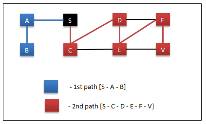
Depth First Search
In this,
- Start at node S.
- Visit A
- Visit B
- Backtrack to A as B don’t have any child nodes
- Backtrack to S as A don’t have any unvisited child nodes
- Backtrack to node S
- Visit C
- Visit D
- Visit E
- Visit F
- Visit V – reached searching node so exit.
The path to node V from S is “S – C – D – E – F – V” and the length of it is 5. In the same graph, using BFS the path we found was “S – C – E – V” and the length of it is 3. So based on this observation, we could say DFS finds a path but it may or may not be a shorted path from source to target node.
Few of advantages of this approach are,
- The fastest way to find a path – it may not be a shortest one.
- If the probability of target node exists in the bottom levels. In an organization chart, if we plan to search a less experienced person (hopefully he will be in bottom layers), the DFS will find him faster compared to BFS because it explores the child nodes lot earlier compared to BFS.
DFS implementation
We can implement this in multiple ways. One is using the recursion and other is using Stack data structure. Following is the java implementation of this algorithm.
   public static void graphDFSByRecersion(Node<String> currentNode) {
    if (null == currentNode) {
      return; // back track
    }
    visitNode(currentNode);
    currentNode.visited = true;
    //check if we reached out target node
    if (currentNode.equals(targetNode)) {
      return; // we have found our target node V.
    }
    //recursively visit all of unvisited neighbors
    for (Node<String> neighbor : currentNode.neighbors) {
      if (!neighbor.visited) {
        graphDFSByRecersion(neighbor);
      }
    }
  }

  public static void graphDFSByStack(Node<String> source) {
    //if empty graph, return
    if (null == source) {
      return; //
    }
    Stack<Node<String>> stack = new Stack<Node<String>>();
    //add source to stack
    stack.push(source);
    while (!stack.isEmpty()) {
      Node<String> currentNode = stack.pop();
      visitNode(currentNode);
      currentNode.visited = true;
      //check if we reached out target node
      if (currentNode.equals(targetTreeNode)) {
        return; // we have found our target node V.
      }
      //add all of unvisited nodes to stack
      for (Node<String> neighbor : currentNode.neighbors) {
        if (!neighbor.visited) {
          stack.push(neighbor);
        }
      }
    }
  }

  public static void treeDFSByRecersion(Node<String> currentNode) {
    if (null == currentNode) {
      return; // back track
    }
    visitNode(currentNode);
    //check if we reached out target node
    if (currentNode.equals(targetNode)) {
      return; // we have found our target node V.
    }
    //recursively visit all of unvisited neighbors
    for (Node<String> neighbor : currentNode.neighbors) {
              graphDFSByRecersion(neighbor);
    }
  }

  public static void treeDFSByStack(Node<String> source) {
    //if empty graph, return
    if (null == source) {
      return; //
    }
    Stack<Node<String>> stack = new Stack<Node<String>>();
    //add source to stack
    stack.push(source);
    while (!stack.isEmpty()) {
      Node<String> currentNode = stack.pop();
      visitNode(currentNode);
      //check if we reached out target node
      if (currentNode.equals(targetTreeNode)) {
        return; // we have found our target node V.
      }
      //add all of unvisited nodes to stack
      for (Node<String> neighbor : currentNode.neighbors) {
          stack.push(neighbor);
      }
    }
  }

Following is the full sample code in Java and you can download and play with the code.

package com.sada.graph;

import java.util.ArrayList;
import java.util.HashMap;
import java.util.HashSet;
import java.util.LinkedList;
import java.util.List;
import java.util.Queue;
import java.util.Set;
import java.util.Stack;

//@author Sada Kurapati <sadakurapati@gmail.com>
public class GraphTraversals {

  public static final Node<String> targetNode = new Node<String>("V");
  public static final Node<String> targetTreeNode = new Node<String>("D");

  public static void main(String args[]) {
    //build sample graph.
    Node<String> source = getSampleGraph();
    Node<String> root = getSampleTree();
    //graphBFSByQueue(source);
    //graphBFSByLevelList(source);
    //treeBFSByQueue(root);
    //treeBFSByLevelList(root);
    //graphDFSByRecersion(source);
    //graphDFSByRecersion(source);
    //treeDFSByRecersion(root);
    treeDFSByStack(root);

  }

  public static void graphBFSByQueue(Node<String> source) {
    //if empty graph, then return.
    if (null == source) {
      return;
    }
    Queue<Node<String>> queue = new LinkedList<Node<String>>();
    //add source to queue.
    queue.add(source);
    visitNode(source);
    source.visited = true;
    while (!queue.isEmpty()) {
      Node<String> currentNode = queue.poll();
      //check if we reached out target node
      if (currentNode.equals(targetNode)) {
        return; // we have found our target node V.
      }
      //Add all of unvisited neighbors to the queue. We add only unvisited nodes to avoid cycles.
      for (Node<String> neighbor : currentNode.neighbors) {
        if (!neighbor.visited) {
          visitNode(neighbor);
          neighbor.visited = true; //mark it as visited
          queue.add(neighbor);
        }
      }
    }
  }

  public static void graphBFSByLevelList(Node<String> source) {
    //if empty graph, then return.
    if (null == source) {
      return;
    }
    Set<Node<String>> frontier = new HashSet<Node<String>>();
    //this will be useful to identify what we visited so far and also its level
    //if we dont need level, we could just use a Set or List
    HashMap<Node<String>, Integer> level = new HashMap<Node<String>, Integer>();
    int moves = 0;
    //add source to frontier.
    frontier.add(source);
    visitNode(source);
    level.put(source, moves);
    while (!frontier.isEmpty()) {
      Set<Node<String>> next = new HashSet<Node<String>>();
      for (Node<String> parent : frontier) {
        for (Node<String> neighbor : parent.neighbors) {
          if (!level.containsKey(neighbor)) {
            visitNode(neighbor);
            level.put(neighbor, moves);
            next.add(neighbor);
          }
          //check if we reached out target node
          if (neighbor.equals(targetNode)) {
            return; // we have found our target node V.
          }
        }//inner for
      }//outer for
      moves++;
      frontier = next;
    }//while
  }

  public static void treeBFSByQueue(Node<String> root) {
    //if empty graph, then return.
    if (null == root) {
      return;
    }
    Queue<Node<String>> queue = new LinkedList<Node<String>>();
    //add root to queue.
    queue.add(root);
    while (!queue.isEmpty()) {
      Node<String> currentNode = queue.poll();
      visitNode(currentNode);
      //check if we reached out target node
      if (currentNode.equals(targetTreeNode)) {
        return; // we have found our target node V.
      }
      //Add all of unvisited neighbors to the queue. We add only unvisited nodes to avoid cycles.
      for (Node<String> neighbor : currentNode.neighbors) {
        queue.add(neighbor);
      }
    }
  }

  public static void treeBFSByLevelList(Node<String> root) {
    //if empty graph, then return.
    if (null == root) {
      return;
    }
    List<Node<String>> frontier = new ArrayList<Node<String>>();
    //add root to frontier.
    frontier.add(root);
    while (!frontier.isEmpty()) {
      List<Node<String>> next = new ArrayList<Node<String>>();
      for (Node<String> parent : frontier) {
        visitNode(parent);
        //check if we reached out target node
        if (parent.equals(targetTreeNode)) {
          return; // we have found our target node V.
        }

        for (Node<String> neighbor : parent.neighbors) {
          next.add(neighbor);
        }//inner for
      }//outer for
      frontier = next;
    }//while
  }

  public static void graphDFSByRecersion(Node<String> currentNode) {
    if (null == currentNode) {
      return; // back track
    }
    visitNode(currentNode);
    currentNode.visited = true;
    //check if we reached out target node
    if (currentNode.equals(targetNode)) {
      return; // we have found our target node V.
    }
    //recursively visit all of unvisited neighbors
    for (Node<String> neighbor : currentNode.neighbors) {
      if (!neighbor.visited) {
        graphDFSByRecersion(neighbor);
      }
    }
  }

  public static void graphDFSByStack(Node<String> source) {
    //if empty graph, return
    if (null == source) {
      return; //
    }
    Stack<Node<String>> stack = new Stack<Node<String>>();
    //add source to stack
    stack.push(source);
    while (!stack.isEmpty()) {
      Node<String> currentNode = stack.pop();
      visitNode(currentNode);
      currentNode.visited = true;
      //check if we reached out target node
      if (currentNode.equals(targetTreeNode)) {
        return; // we have found our target node V.
      }
      //add all of unvisited nodes to stack
      for (Node<String> neighbor : currentNode.neighbors) {
        if (!neighbor.visited) {
          stack.push(neighbor);
        }
      }
    }
  }

  public static void treeDFSByRecersion(Node<String> currentNode) {
    if (null == currentNode) {
      return; // back track
    }
    visitNode(currentNode);
    //check if we reached out target node
    if (currentNode.equals(targetNode)) {
      return; // we have found our target node V.
    }
    //recursively visit all of unvisited neighbors
    for (Node<String> neighbor : currentNode.neighbors) {
              graphDFSByRecersion(neighbor);
    }
  }

  public static void treeDFSByStack(Node<String> source) {
    //if empty graph, return
    if (null == source) {
      return; //
    }
    Stack<Node<String>> stack = new Stack<Node<String>>();
    //add source to stack
    stack.push(source);
    while (!stack.isEmpty()) {
      Node<String> currentNode = stack.pop();
      visitNode(currentNode);
      //check if we reached out target node
      if (currentNode.equals(targetTreeNode)) {
        return; // we have found our target node V.
      }
      //add all of unvisited nodes to stack
      for (Node<String> neighbor : currentNode.neighbors) {
          stack.push(neighbor);
      }
    }
  }

  public static void visitNode(Node<String> node) {
    System.out.printf(" %s ", node.data);
  }

  public static Node<String> getSampleGraph() {
    //building sample graph.
    Node<String> S = new Node<String>("S");
    Node<String> A = new Node<String>("A");
    Node<String> C = new Node<String>("C");
    Node<String> B = new Node<String>("B");
    Node<String> D = new Node<String>("D");
    Node<String> E = new Node<String>("E");
    Node<String> F = new Node<String>("F");
    Node<String> V = new Node<String>("V");

    S.neighbors.add(A);
    S.neighbors.add(C);

    A.neighbors.add(S);
    A.neighbors.add(B);

    B.neighbors.add(A);

    C.neighbors.add(S);
    C.neighbors.add(D);
    C.neighbors.add(E);

    D.neighbors.add(C);
    D.neighbors.add(E);
    D.neighbors.add(F);

    E.neighbors.add(C);
    E.neighbors.add(D);
    E.neighbors.add(F);
    E.neighbors.add(V);

    F.neighbors.add(D);
    F.neighbors.add(E);
    F.neighbors.add(V);

    V.neighbors.add(E);
    V.neighbors.add(F);

    return S;
  }

  public static Node<String> getSampleTree() {
    //building sample Tree.
    Node<String> A = new Node<String>("A");
    Node<String> B = new Node<String>("B");
    Node<String> C = new Node<String>("C");
    Node<String> D = new Node<String>("D");
    Node<String> E = new Node<String>("E");
    Node<String> F = new Node<String>("F");
    Node<String> G = new Node<String>("G");
    Node<String> H = new Node<String>("H");

    A.neighbors.add(B);
    A.neighbors.add(C);
    A.neighbors.add(D);

    B.neighbors.add(E);
    B.neighbors.add(F);
    B.neighbors.add(G);

    C.neighbors.add(H);

    return A;
  }

}

class Node<T> {

  T data;
  ArrayList<Node<T>> neighbors = null;
  boolean visited = false;

  Node(T value) {
    data = value;
    neighbors = new ArrayList<Node<T>>();
  }

  @Override
  public int hashCode() {
    int hash = 5;
    return hash;
  }

  @Override
  public boolean equals(Object obj) {
    if (obj == null) {
      return false;
    }
    if (getClass() != obj.getClass()) {
      return false;
    }
    final Node<?> other = (Node<?>) obj;
    if (this.data != other.data && (this.data == null || !this.data.equals(other.data))) {
      return false;
    }
    return true;
  }
}


